Thinking of linear programs geometrically
Table of Contents
Representing a two-variable LP graphically
Consider the following linear program:
Maximize \(x+y\)
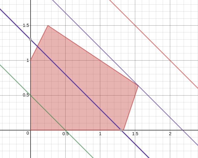
subject to \[\begin{aligned} 2x+3y & \le 5 \\ -2x+ y & \le 1 \\ 3x- y & \le 4 \\ x, y & \ge 0 \end{aligned}\]
We can represent this graphically in the \(xy\)-plane. For each constraint, the set of points \((x,y)\) that satisfies it is a half-plane; the set of points satisfying all of the constraints is then the intersection of all these half planes. In this example it turns out to be a pentagon, shaded red in the image below.
The set of points that satisfy all the constraints is called the feasible region. It is always convex, meaning that whenever two points are in the feasible region, so is the entire line segment connecting them. It doesn’t have to be of finite size as it is for this linear program, it can “go off to infinity”. It can also be empty! (It is a good exercise to draw half-planes that would give a feasible region of infinite extent, and to draw half-plane that don’t have any point common to all, leading to an empty feasible region.)
How can we represent the objective function? The graph of the function would require three dimensions to plot (i.e., the graph is the plane \(z=x+y\) in three-dimensional space). To get something we can draw in the same figure as the feasible region we will instead draw level curves \(x+y = k\) that you get by setting the objective function equal to a constant \(k\). (Since the objective function is linear these level “curves” are actually straight lines.)
Here is a picture of the feasible region together with various level lines for the objective function:
As you change the constant \(k\), the level line slides around, always keeping the same slope. If for some value of \(k\) that line goes through the feasible region, that means that it is possible to obtain the value \(k\) for some choice of \(x\) and \(y\) satisfying the constraints. We want the largest such \(k\), so imagine sliding the line around until it is about to fall off the feasible region: the corresponding \(k\) is the maximum1 value of the objective function in the feasible region and the answer to the optimization question posed by the linear problem.
Explore the example interactively with Desmos
If you’re reading this on a computer2 you’re in luck: using the lovely online graphing tool Desmos you can explore the above example interactively.
- Here’s a picture of just the constraints. Each one is drawn as a translucent half-plane, where the half-planes overlap their colors combine. You can turn each constraint on and off by clicking on the colored circle next to the inequality in the left-hand column.
- Here’s a picture of the feasible region3 with a movable level line for the objective function. Play with the slider to approximately maximize the objective function!
Why don’t we just always do this?
For the example above this graphical way of thinking works wonderfully: we see right away that the optimal solution is at the point where the two constraints \(2x+3y \le 5\) and \(3x - y \le 4\) both turn into equalities. Solving the system of equations we get \( x = 17/11, y = 7/11\), so the maximum of the objective function is \(24/11\).
But this isn’t a practical method in general. This LP had only two variables so our picture was two-dimensional. Natural LPs tend to have many, many more variables and geometric intuition tends to give out after three dimensions!
Or minimum, depending on which side it’s falling off! In this example clearly the minimum is 0, attained at the origin.
If you are reading this on paper, I apologize.
Notice the way all the constraints are combined into one to get the feasible region. This is just because there doesn’t seem to currently be a way of asking Desmos to intersect various regions.